Gated PixelCNN

Written 24 Feb 2017 by Sergei Turukin

This is a follow-up post of this one. Here I’ll continue to describe my struggle implementing Conditional Gated PixelCNN.

In a paper authors improve PixelCNN model in several ways:

1. Replace relu activations with gated block: sigmoid and tanh
2. Eliminate blind spot in receptive field
3. Add global conditioning

In this blog post I’ll describe how I had implemented those. Again, I’ll continue using chainer as my implementation framework.

Note: You can find source code of my implementation in github.

Gated blocks

As the very first step authors replaced relu activation block with more complex combination of sigmoid (as a forget gate) and tanh (as real activation). Authors suggest that this could be one reason PixelRNN (that used LSTM’s) outperformed PixelCNN. They used \(\mathbf{y} = tanh(W_{k,f} \ast \mathbf{x}) \odot \sigma(W_{k,g} \ast \mathbf{x})\) as activation function (block, actually) instead of relu. Refer to original paper for details.

In paper they combine convolutions for sigmoid and tanh gates into one operation for speed and split feature maps after (before applying activations). That is pretty simple when there is no channel masking, but I was unable to think of split solution for channel masking and went with two separate convolutions.

Blind spots

Let us continue with blind spots next. I’ll try to explain why and how they acutally appear. Recall, that we were using masks to disable wrong information (infotmation from ‘future’ pixels) get to one we’re interested in. That is what our convolution weight matrix mask looks like (for 5x5 filter):

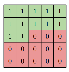
Now let’s think about what information layer L gets from layer L-1. Basically, all green (in a picture above) pixels will contribute while red won’t. Next step is to go deeper one level and ask yourself what information those pixels posess. Other words, what information layer L gets from L-2 layer? We’re particularly interested in rightmost pixels as they extend our receptive field. What we see is that due to masking they won’t have access to some pixels layer L interested in. If we continue our logic it’s clear that layer L ‘does not see’ some pixels. Here is animation for that case.

Animation above shows what L-2 layer pixels are seen from L layer point of view.

As you can observe yellow pixel is not seen! But it should be accessible because it is ‘previous’: it’s above current (center) one.

Checking with code

Following code snippet will try to conivnce your there is blind spot if you still aren’t.

# create 5x5 input
# chainer requires input to have shape [BATCH, CHANNELS, HEIGHT, WIDTH]
input = np.arange(25).reshape([1,1,5,5]).astype('f')
# array([[[[    0.,     1.,     2.,     3.,     4.],
#          [    5.,     6.,     7.,     8.,     9.],
#          [   10.,    11.,    12.,    13.,    14.],
#          [   15.,    16.,    17.,    18.,    19.],
#          [   20.,    21.,    22.,    23.,    24.]]]], dtype=float32)

# create kernel of ones so it just sums all values within
# use one for simplicity: easy to check
kernel = np.ones([3, 3])
# turn to proper type 'A' mask
kernel[2:, :] = 0.0
kernel[1, 1:] = 0.0
# array([[ 1.,  1.,  1.],
#        [ 1.,  0.,  0.],
#        [ 0.,  0.,  0.]])

# create two convolution layers with total receptive field size 5x5
# so out input is exact fit
import chainer.links as L

l1 = L.Convolution2D(1, 1, ksize=3, initialW=mask)
l2 = L.Convolution2D(1, 1, ksize=3, initialW=mask)

# here is the trick: pixel at [1, 4] position will be inside blind spot
# if we perform convolution its value won't be included in final sum
# so let's increase its value so it would be easy to check
input[:, :, 1, 4] = 1000
# array([[[[    0.,     1.,     2.,     3.,     4.],
#          [    5.,     6.,     7.,     8.,  1000.],
#          [   10.,    11.,    12.,    13.,    14.],
#          [   15.,    16.,    17.,    18.,    19.],
#          [   20.,    21.,    22.,    23.,    24.]]]], dtype=float32)

output = l2(l1(input)).data
# array([[[[ 64.]]]], dtype=float32)
# Viola! Sum is lesser that 1000 which means pixel at [1, 4] wasn't seen!

# Otherwise, let's return it value back
input[:, :, 1, 4] = 9
# array([[[[    0.,     1.,     2.,     3.,     4.],
#          [    5.,     6.,     7.,     8.,     9.],
#          [   10.,    11.,    12.,    13.,    14.],
#          [   15.,    16.,    17.,    18.,    19.],
#          [   20.,    21.,    22.,    23.,    24.]]]], dtype=float32)

# perform computation again..
output = l2(l1(input)).data
# array([[[[ 64.]]]], dtype=float32)
# Another evidence: no matter what value we assign to it final sum doesn't change
# That proves it's within blind spot and we can't access information at it.

Stacks

Ok. Hope you’re convinced now. How do we eliminate this nasty blind spot? How do we make our model access all pixels it’s interested in? Authors introduce neat idea: they split convolution into two different operations: two separate stacks - vertical and horizontal.

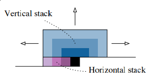
Here we have horizontal stack (in purple): convolution operation that conditions on only current row, so it has access to left pixels. Vertical stack (blue) has access to all top pixels. Implementation details would follow.

Note that horizontal and vertical stacks are sort of independent: vertical stack should not access any information horizontal stack has: otherwise it will have access to pixels it shouldn’t see. But vertical stack can be connected to vertical as it predicts pixel following those in vertical stack. Next image (taken from original paper) illustrates how stacks are connected.

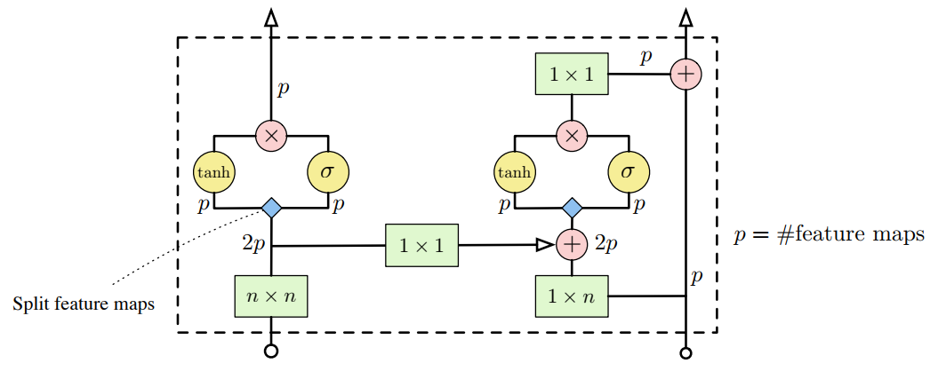
Please note that convolution operations (in green) are masked!

This didn’t actually helped me to understand how should one really implement those 1xn and nxn convolutions (that should be masked!). But Reed et al, 2017 brought some insights of how it can be done. Also I found this implementation really helpful (read comments in pixelConv layer implementation).

Base thing that one should grasp is that after performing those convolutions information from pixels considered ‘future’ should not pass into current (center). Then it’s up to implementation how to achieve that. I take approach from Reed paper with padding, cropping and shifting.

Horizontal stack

Consider horizontal stack at first. Suggested idea is to perfrom 1 x n//2 + 1 convolution with shift (pad and crop) rather than 1 x n masked convolution. What you basically do is convolve the row with a kernel of slightly different width (2 instead of 3 or 4 instead of 7) with padding and cropping output so the shape stays the same. Having limited filter size is equivalent of masking. Compare these two operations (upper image convolve with kernel width of 2 and without masks, bottom - kernel width of 3 and applies mask):

One thing to remember is that for mask type ‘A’ we still have to perform masking convolution as otherwise predicted pixel information will seep into our model and conditional distribution would not be modelled correctly. Other way to implement this sort of masking without actually applying masks (via matrix multiplication) is to pad’n’crop input more. This is equivalent to output shifting.

That image shows us that last sample from output (just before ‘Crop here’ line) doesn’t have information flow from last input sample (dashed line). Kernel width we’re using here is 2, no masks used (dashed line just illustrates there is no real connection).

Vertical stack

Next to vertical stack. In order to obtain receptive field size that grows in rectangular fashion without touching ‘future’ pixels one could use same trick with padding, convolving with slightly different kernel height (we’re implementing vertical stack now) and cropping to force output depend only on upper pixels.

So I again took kernel size to be n//2 + 1 x n instead of n x n, padded input at top, perform convolution operation, then cropped output to preserve spatial dimensions. One can easily check that in that case first row of output doesn’t contain any information from the same row of input, only on previous 2 (in case we have n=3) rows. We don’t need any masking here as no target pixel is touched (it always takes information from top pixels and sends that info to horizontal stack where all other magic happens).

In the animation above we pad input (left) with kernel height zeros, perform convolution and then crop output so that rows are shifted by one with respect to input. One can notice that first row of output doesn’t depend on first (real, non-padded) input row. Second row of oupput depends only on first input row. We’ve got desired behaviour.

A little of coding

# our convolution kernel
kernel = np.ones([2, 3])
# array([[ 1.,  1.,  1.],
#        [ 1.,  1.,  1.]])

# create our input image and pad it
input = np.arange(25).reshape([1,1,5,5]).astype('f')
padded = np.pad(input, [(0, 0), (0, 0), (2, 2), (1, 1)], 'constant')
# array([[[[  0.,   0.,   0.,   0.,   0.,   0.,   0.],
#          [  0.,   0.,   0.,   0.,   0.,   0.,   0.],
#          [  0.,   0.,   1.,   2.,   3.,   4.,   0.],
#          [  0.,   5.,   6.,   7.,   8.,   9.,   0.],
#          [  0.,  10.,  11.,  12.,  13.,  14.,   0.],
#          [  0.,  15.,  16.,  17.,  18.,  19.,   0.],
#          [  0.,  20.,  21.,  22.,  23.,  24.,   0.],
#          [  0.,   0.,   0.,   0.,   0.,   0.,   0.],
#          [  0.,   0.,   0.,   0.,   0.,   0.,   0.]]]], dtype=float32)

# convolve it and crop
l = L.Convolution2D(1,1, ksize=(2,3), initialW=kernel)
l(padded)[:, :, :-2, :].data
# array([[[[   0.,    0.,    0.,    0.,    0.],
#          [   1.,    3.,    6.,    9.,    7.],
#          [  12.,   21.,   27.,   33.,   24.],
#          [  32.,   51.,   57.,   63.,   44.],
#          [  52.,   81.,   87.,   93.,   64.],
#          [  72.,  111.,  117.,  123.,   84.]]]], dtype=float32)

# compare to our pre-padded input:
# array([[[[  0.,   1.,   2.,   3.,   4.],
#          [  5.,   6.,   7.,   8.,   9.],
#          [ 10.,  11.,  12.,  13.,  14.],
#          [ 15.,  16.,  17.,  18.,  19.],
#          [ 20.,  21.,  22.,  23.,  24.]]]], dtype=float32)

# As we can see first output row doesn't have any information from first input row
# second row has only information from first but not the second input row, etc.

Other implementation tricks

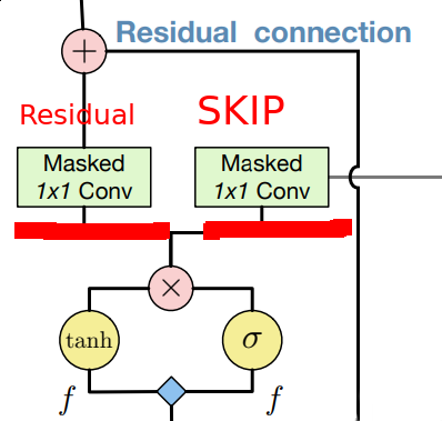
Two important mentions here: do not forget about residual and skip connections. One uses residual connections only for horizontal stack (paper authors state using them for vertical doesn’t help much).

On the other side skip connections allow as to incorporate features from all layers at the very end of out network. Most important stuff to mention here is that skip and residual connection use different weigths after gated block.

I actually found that Reed paper offers more clear and thourough explanation of how block should be implemented. Also, they propose 1 x n followed by n x 1 instead of n x n convolution in vertical stack along with other neat tricks. It’s definitely a good complementary read!

Conditioning

Now on to conditioning. Conditioning is a smart word for saying that we’re feeding out network some high-level information. Think about classes in MNIST/CIFAR datasets. During training you feed image as well as class to your network to make sure network would learn to incorporate that information as well. During inference you can specify what class your output image should belong to.

You can pass any information you want with conditioning, we’ll start with just classes.

For that we modify our block to include information to condition on like this:

Note \(\mathbf{h}\) multiplied by matrix inside tanh and sigmoid functions. I used simple embedding, so my V matrix had shape [number of classes, number of filters]. I passed class as one-hot vector during training and inference.

Coding session

To better understand how should we incorporate conditioning information consider this snippet.

# Let's say here is our output after convolution at some layer L
# convolution output in chainer has shape [BATCH, CHANNELS, HEIGHT, WIDTH]
output = np.random.rand(1, 32, 10, 10)

# Let's say it's output for MNIST image with label 9 (i.e. it's an image if nine)
label = 9
# convert to one hot encoding - `h`. Total class count - cardinality - is 10
h = np.zeros(10)
h[label] = 1.0
# array([ 0.,  0.,  0.,  0.,  0.,  0.,  0.,  0.,  0.,  1.])

# Our embedding matrix `V` should have shape of [number_of_classes, number_of_filters]
# so in our case the shape is [10, 32]
V = np.random.rand(10, 32)

# We now perform dot product that will add to our convolution output
# think about it as "label bias"
label_bias = V.T.dot(label)

# label_bias.shape is (32,). We have to add this label bias vector to every "pixel"
# so we reshape it to (1, 32, 1, 1) and allow our framework to broadcast it

output = output + np.reshape(label_bias, [1, 32, 1, 1])

One could extend conditioning and make it position-dependent as author state in paper (last paragraph of section 2.3) but I didn’t do that. I was unwilling to increase computation cost even further and wanted to get to Wavenet as soon as possible.

Results

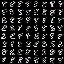
Very first results i was getting after couple minutes of training with simplified architecture (othwerwise it takes too much time). I limited model to have 5 blocks, 128 hidden dimensions, 16 hidden output dimenstions and 4-way softmax. Here results for MNIST dataset generation for label 7:

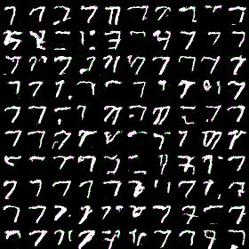
Looks prettty good: i definitely can discern sevens here and they’re pretty diverse.

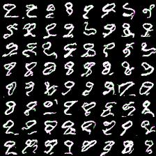
Similiar results (with same architecture) for longer training (25 epoch vs 1, ~1 hour vs 2-3 minutes), label is 1:

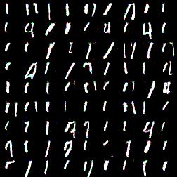
That looks even better! More clear ones, interestingly there are some fours as well. That’s is not good but nevertheless interesing: they have similiar shape. I wonder why there are no sevens.

You know, I really liked MNIST dataset for its simplicity and quick iteration cycle. This is the main reason I always tend to use 4-or-8-way softmax (that is, only 4 or 8 pixel values) instead of full-blown 256-way softmax. Training time numbers I was able to recover from paper are:

(60 hours using 32 GPUs)

Not very promising ;(

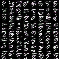
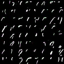
My best results with 256-way softmax (and MNIST) after 12 hours of training on one NVIDIA GTX Titan X (Pascal) are below. These were generated with network of 8 blocks, 128 hidden dimensions, 16 output hidden dimensions, first image is generated at 100k iterations, second - 500k.

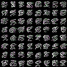
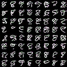
It’ clear that first sample images are quite wiggly but situation improves with more training time. Second one look better and start resemble eights (condition label was 8 in both cases).

[01.03.17: update] results

I was really not very satsified with results (is the model is wrong or my hyperparameters were bad or traiing process is flawed?) and conducted a series of experiments to see how the model is doing.

I want to mention that during writing this post I realized i had wrong first layer implementations for gated block. I changed the code it to my best understanding but I’m still not sure if it was fixed.

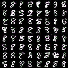
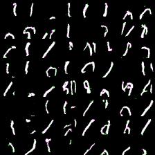
However, here i present results of my attempts to convince myself everything is ok. First series of experiment include weight_decay (L2 weight regularizer) and gradient L2 norm clipping to facilitate training and get rid of loss function spikes. Below are results for MNIST dataset with default settings, trained for 20 epochs (couple of hours training). First (rightmost) image corresponds to 8-way softmax, center - 16-way, rightmost - 32-way. Results are pretty good in my opinion (nice looking eights).

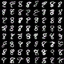
Thing to mention is that it’s harder to train more complex model (softmax with more outputs: 128, 258). Next results demonstrate this. I was experimenting with 64- and 128-way softmaxes. Right images are for 64-way softmax, left - 128. Top images have label conditioning of 8, bottom - 1. Training time is equal for both models - 20 epochs (again couple of hours).

Again, more complex model produces less impressive results (if impresive at all) and requires mode time to train. However, they at least able to differentiate between eights and ones.

References

Most helpful and influential links for me were:

• Keras/theano implementation
• Reed paper