PixelCNN
Some time ago Google’s Deepmind team announced of getting good audio generation results with their recent Wavenet model. That was particularly interesting for me and for educating and research purposes I decided to replicate their study (at least some parts of it) and implement WaveNet model by myself. In this post I’ll start my journey of implementing it.
After reading paper first time it was clear to me that for reduce my total misunderstanding of a paper I should go first to PixelCNN paper as Wavenet architecure (and paper itself) is based on it. So, straight to PixelCNN.
Little theory
Main purpose of PixelCNN model is to model (apology for tautology) pixel distribution \(p(\mathbf{x})\), where \(\mathbf{x} = (x_0, .., x_n)\) vector if pixel values of given image. Authors employ autoregressive models to do that: they just use plain chain rule for joint distribution: \(p(\mathbf{x}) = p(x_0)\prod_1^n p(x_i \vert x_{i<})\). So the very first pixel is independent, secodnd depend on first, third depends on first and second and so on. Basically you just model your image as sequence of points (think of time series) where each one depends linearly on previous ones.
One consequence of such modeling is that it somewhat constrains inference: generation should be performed sequentially: you generate first pixel with one forward pass, then generate second one given the first and continue the process until you have whole image generated. That is in contrast with convolutional neural network where the whole process is sort of parallel (kernel working on an image).
Implementation details
Note: You can find source code of my implementation in github.
As a side note I want to mention that as implementing PixelCNN paper is just a prerequisite to WaveNet and therefore I focus solely on convolutional implementation and ignore recursive variants of PixelRNN. Most implementations I’ve found on the internet (see whole list i’ve considered mot helpful and influential in last section of post) devote more attetion RNN’s, but I’m inclined more to CNN variant.
As another note, I want’ to mention that digging information from research papers is kind of black art and having ton of experience could help you to fill information gaps (that’s not my case, unfortunately). In order to implement most basic variant of a model I had to spend some time reading all somehow related papers, going through existing (not always correct and complete) implementations and others.
Framework
Implementation of PixelCNN is done with chainer. I was using tensorflow before and found chainer to be better suited for quick-and-dirty approach to experiment and for paper implementation.
Modeling conditional independence
PixelRNN introduces notion of masks as a convenient way of enforcing dependecies between pixels.
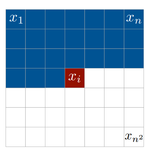
Here pixel \(x_i\) depends on pixels \(x_1 .. x_{i-1}\) so we have to ensure it won’t access all ‘subsuequent’ pixels: \(x_{i+1} .. x_n^2\). Masks is a good way to achieve that: all we need to do is to provide mask that block information flow from that pixels (more on that later).
I want to note that particular ordering is comfortable to think about (right-to-left, top-to-bottom), at least for West-minded people. But order can be pretty arbitrary as stated in Masked Autoencoder for Distribution Estimation.
Architecture
Here is final diagram used for PixelCNN model implemented. h is number of hidden channels, d is number of output hidden channels. In illustration I used chainer way to specify convolution weights shape, namely: [Number of output channels, number of input channels, kernel height, kernel width].
![]()
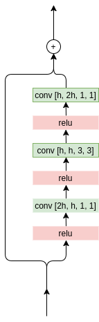
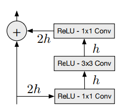
And here is how residual block looks like:
Througout the model spatial dimenstions are preserved: padding is chosen to keep dimensions the same.
As illustrated it has first convolution layer with mask type ‘A’ (more about masks later) that means center pixel in mask is zeroed, i.e. we guarantee model won’t get access to pixel it is about to predict. This is really obvious: if we allow pixel-to-be-predicted to be connected to our model then the best way to predict its value in the last layer is to learn to mimic it (think making center weight equal to one and all others to zero). Zeroing center pixel in first layer mask breaks this convenient information flow and forces the model to learn to predict the pixel based on previous inputs.
Residual blocks
Residual block would be changed later when we implement Gated PixelCNN - inspiration from PixelRNN LSTM blocks with memory. For now it’s just 3 subsequent convolutons: first one halves the number of filters (I’m thinking reduce computational cost has something to do with that), next one is ‘regular’ 3x3 convolution preserving number of filters followed by another one 1x1 convolution to restore filters back to original size. Convolutions have relu activation functions interspersed.
There is one thing regarding activation functions within block: it wasn’t very obvious for me how relu’s should be placed: image in a paper is quite confusing. Should be relu’s be placed before convolutions or should we follow traditional approach described in He et al, 2015?
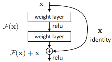
My initial approach was to follow He’s approach but changed my mind in the middle of process when my model wasn’t learning anything useful and I was experimenting with options. Then I placed relu activations before convolutions and sticked to that decision afterwards. As soon as my model was working I didn’t try to go back to my original version. In a retrospect I’m not thinking there is big difference between two.
Masks
Other thing I want to dedicate some time to are masking. As I had already said masks - are way to restrict information flow from ‘future’ pixels into one we’re predicting. But how do we implement them?
One way (described in a paper) is to use masked convolutions: all we need is just zero out some weights in convolution filters, like that. It is easy to see, that information from pixels below won’t reach target (center) pixel as well as from pixels on the same line to the right of target.

Here illustrated resulting receptive field of two 3x3 masked convolution layers (receptive field size is in that case 5x5). Each input is transparent so we can see that some inputs are taken into account several time (they’re more opaque), but it should be clear that using masks allows us to ignore pixels we don’t want.

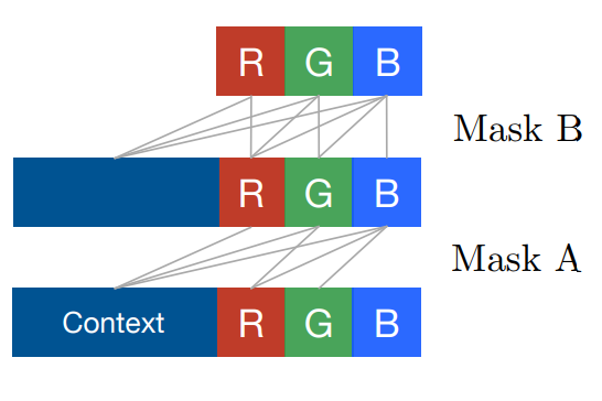
Worth noting that if we’re working with full colored images then masks should be extended. In paper authors actually allow information from R (red) channel go into G (green), and from R and G go into B. So we have ordering not only within spatial dimensions but also within source channels (think colors) too.
Here are some images to better understand how those masks should be implemented (image taken from original paper and shows masks of both types: ‘A’ and ‘B’)
So, ultimately we should split convolution filters (hidden dimensions) into 3 groups: one group for R color, second one is for G channel, third one - for B channel. There basically several ways to do that: first one is to reserve first N / 3 filters to be “red”, next N / 3 - “green”, rest - “blue”. Other is to virtually split filters into groups of 3, each one corresponding to every channel. Images below illustrate that (connections are not shown here):


Either way would work but I personally chose the second way (groups of 3). Now, as we decided what filters corresponds to each color channel we can go on to describe how they should be connected and how to implement masks to achieve that connectivity. As for MADE section 4, masks are a good way to enforce proper computational paths between underlying image colors and filters.
Let first understand how should we implement masks for grayscale (that is, 1 input filter/channel). That case we don’t care about color/channel splitting and concentrate on context masking: make pixel depend only on previous ones and not having any information from next. Code below shows how it could be coded:
filters_output, filters_input, filter_height, filter_width = W.shape
mask = np.ones_like(W).astype('f')
y_center, x_center = filter_height // 2, filter_width // 2

mask[:, :, yc+1:, :] = 0.0
mask[:, :, yc:, xc+1:] = 0.0
Here we have weight matrix W with shape of [Number of output filters, number of input filters, filter height, filter width]. Mask will have same dimensions (as it’s applied to weights before convolution operation). Next we find our center and zero all weight below and right of it. The resulting mask would look like this (for 7x7 convolution):
array([[ 1.,  1.,  1.,  1.,  1.,  1.,  1.],
       [ 1.,  1.,  1.,  1.,  1.,  1.,  1.],
       [ 1.,  1.,  1.,  1.,  1.,  1.,  1.],
       [ 1.,  1.,  1.,  0.,  0.,  0.,  0.],
       [ 0.,  0.,  0.,  0.,  0.,  0.,  0.],
       [ 0.,  0.,  0.,  0.,  0.,  0.,  0.],
       [ 0.,  0.,  0.,  0.,  0.,  0.,  0.]])
Note that our center pixel is zero. This corresponds to mask type ‘A’: next layer output don’t have information for a pixel it tries to predict. We use that sort of mask only for first layer: there is no sense to block information flow aftewards.
This masks encode spatial (context) masking. Now, we step up to color masks to perform color masking. We now modify masks to change first two dimensions of our weights matrix: only filter weights are affected: W[:, :, y_center, x_center].


As we see, we should allow connections from R channel to G and B and from G to B. For mask type ‘B’ we also allow connection from R to R, B to B, G to G. Let’s assume we have 4 input filters and 7 output (just to show how we deal with numbers of filters that is not strictly divisible by 3).
Image below shows how our filters should be connected (for mask type ‘A’ to reduce number of connections).

Our weight matrix for center weight mask type ‘A’ (y_center, x_center = 3, 3 in case of 7x7 convolution) would look like this (rows are for output filters, columns - input):
array([[ 0.,  0.,  0.,  0.],
       [ 1.,  0.,  0.,  1.],
       [ 1.,  1.,  0.,  1.],
       [ 0.,  0.,  0.,  0.],
       [ 1.,  0.,  0.,  1.],
       [ 1.,  1.,  0.,  1.],
       [ 0.,  0.,  0.,  0.]])
Here we can see, that first, fourth and seventh rows (filters, corresponding to output R channel) are zeroed because we don’t allow R channel filter to have acces to any information (only context). Second and fifth rows have access to first and fourth columns (ones at that positions) because B channel filters can access only R channels. Finally, 3rd and 6th rows connected to 1st, 2nd, 4th rows as B channel filter can access both R and B channels.
If we are about to see how mask ‘B’ would look like then we should recall that then we allow R output filters have acces to R input filter, B - to B, G - to G. Resulting weight matrix (again, for center pixel only) would look like:
array([[ 1.,  0.,  0.,  1.],
       [ 1.,  1.,  0.,  1.],
       [ 1.,  1.,  1.,  1.],
       [ 1.,  0.,  0.,  1.],
       [ 1.,  1.,  0.,  1.],
       [ 1.,  1.,  1.,  1.],
       [ 1.,  0.,  0.,  1.]])
Note ones at positions (0, 0), (0, 3), (1, 1), (4, 1), (2, 2) and so on. Exact implementation of masked convolutions (and masks computation) could be found in my wavenet repository, file wavenet/models.py#L21.
Data preprocessing
As stated in paper they treat output values as categories: that is each pixel each channel output is number (category) between 0 and 255 (we can use any number here, 256 is chosen because RGB is 8 bit).
Input data is preprocessed to be in [0; 1] range for every channel. chainer only applies rescale operation for both MNIST and CIFAR-10 datasets. Input were ‘categorized’ then to labels. [0; 1] range was divided into bins and real values were converted into bin number. This code explains how we transform real values (in zero-one range) to categories (labels):
levels = 256
def quantisize(images, levels):
    return (np.digitize(images, np.arange(levels) / levels) - 1).astype('i')

images = np.random.rand(10)
# array([ 0.63088284,  0.38492999,  0.24928341,  0.38114789,  0.22476074,
#         0.05843769,  0.93718617,  0.50012818,  0.06850125,  0.04906324])

quantisize(images, 256)
# array([161,  98,  63,  97,  57,  14, 239, 128,  17,  12], dtype=int32)

# First 10 bins
(np.arange(levels) / levels)[:10]
# array([ 0.        ,  0.00390625,  0.0078125 ,  0.01171875,  0.015625  ,
#         0.01953125,  0.0234375 ,  0.02734375,  0.03125   ,  0.03515625])

# pixel with value between 0 and  0.00390625 gets assigned to 0 label (category),
# pixel with value between 0.00390625 and 0.03515625 -  8, etc.
Initially I started with real values as inputs and labels as outputs. However, model didn’t work for me until i switched to binarized MNIST (input are either zero or ones). I don’t have any explanation for that. I really would be grateful for possible explanation of what’s happen in that case and how could it influence learning and training.
My next step was to increase number of categories from 2 (0/1) to 4 (0/1/2/3), 8 (0/1/2/3/4/5/6/7) and, ultimately, 256 (0-255). For that I quantisized my input data (got labels) and then multiplied by discretization step (train.py#L77) effectively replacing arbitrary real values with real values at fixed locations. Here is more detailed explanation:
levels = 4  # for simplicity
data = np.random.rand(10)
# array([ 0.82021865,  0.40114005,  0.70115555,  0.48837238,  0.358867  ,
#         0.15298734,  0.54490917,  0.32857768,  0.28460412,  0.7673152 ])
labels = quantisize(data, levels)
# array([3, 1, 2, 1, 1, 0, 2, 1, 1, 3], dtype=int32)

discretization_step = 1. / (levels - 1)
# 0.3333333333333333

preprocessed_data = labels * discretization_step
# array([ 1.        ,  0.33333333,  0.66666667,  0.33333333,  0.33333333,
#         0.        ,  0.66666667,  0.33333333,  0.33333333,  1.        ])
That worked.
Training tips’n’tricks
I really like iterative approach to get something work. First you start with very simple problem and solve it, then relax your constraints a little and solve a slightly more difficult problem. Otherwise, it’s not that simple for me to figure out what exactly is not working within my model.
I’ve followed quite a simple approach while implementing the model. First, i’ve made sure I’m able to make it work and generate reasonable output for binarized MNIST dataset. For that I used binarize function (see wavenet/utils.py#L16) to convert from grayscale image to zero-or-one input data. Instead of softmax I used sigmoid cross entropy loss function. After having this working (it took a while to fix bugs and find a proper way of data preprocessing) I replaced sigmoid with 2-way softmax cross entoropy loss.
Next step was to increase number of categories: step away from 2-way softmax to N-way (see quantisize function in wavenet/utils.py#24).
Another big step was to introduce notion of input channels (RGB instead of grayscale) and go for CIFAR-10 dataset instead of MNIST. However, I trained for MNIST (converted to RGB) for some time until I was getting good results. Making masks work took a very long time (once I felt I should abandon masks altogether as switching to color masks gave me much worse results). Once 256-way MNIST data with masks we’re as good as very simple (binarized without masks) version, it was finally time for CIFAR-10 training.
Inference
Since PixelCNN is autoregressive model inference happens to be sequential: we have to generate sample by sample. First, we generate image by passing all-zeros to our model. It shouldn’t influence the very first pixel as its value (to be strict R channel value) is modelled to be independent of anything. So, we perform forward pass and obtain distribution for it. Given the distribution we sample a value using sample_from function (see wavenet/utils.py#32). Then we update our image with that value and continue with G channel value. We iterate until we have all pixel values generated.
It’s worth noting that generation would require 3 * HEIGHT * WIDTH model runs (3072 for CIFAR) and it can’t be parallelized. Not very scalable. However, we still can pass a batch to generate several images simultaneously. Stochastic nature of sample_from routine will help us to get different images.
Results
I never trained model for a very long time, since my goal was to advance as quickly as possible. Because of that I only checked if results generated made sense. If that was the case, I moved on. I usually stopped training within 10 epochs.
Here I’m posting some of my intermediate results (that were saved somewhere and I was able to find at the time of post writing).
First result is binarized mnist:
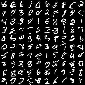
My next step was to increase number of output labels (categories), go from black/white pixels to grayscale. Here is results for 8-way softmax image (note that image is grayscale now).
Next, i wanted to introduce colors: go to RGB images from grayscale. MNIST dataset was converted to RGB before feeding to network. Next result is for 8-way RGB configuration (one can notice some colors due to not perfect model):
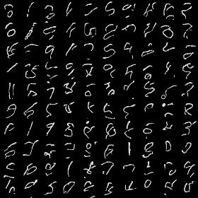
All results above are not bad in my opinion as they at least resemble digits. As I’ve said before proper channel masking took inappropriate amount of time. Basically, i was getting results like that:
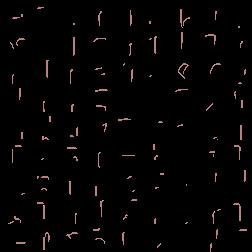
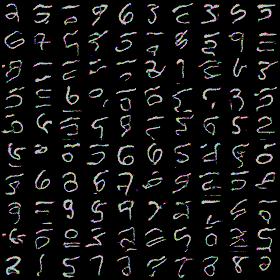
Once masks were correct (I hope) results improved dramatically:
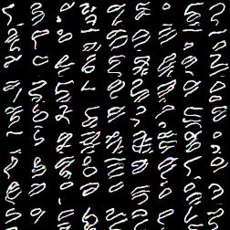 .
.
Though digits look quite wiggly, result is much better than previous one. I haven’t dig into the issue, but during experimenting with simplier model architectures I noticed that training for more time helped me to fix simiar issue. I’m not really sure if this correct explanation. And I can’t locate my best output image for fully-fledged PixelCNN for MNIST dataset, so no proof :)
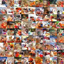
After that I tried to train on CIFAR. I didn’t train for long, but here again results for training for 1 hour with NVIDIA GTX Titan X Pascal. I was pretty happy with that: images look like something and not complete noise. That is already good sign.
What’s next?
Authors have follow-up paper where they show how to improve PixelCNN model to achieve same performance as PixelRNN (which I didn’t implement). They eliminate receptive field blind spot by replacing residual block masked convolutions with separate vertical and horizontal stacks, introduce class conditioning and update convolution operations inside blocks with ‘special’ gated blocks.
In my next post I’ll describe all that stuff.
Resources
Here is a list of resources I’ve found to be extremely helpful for me in my journey to implement PixelCNN.