Wavenet
This is 3rd post in a series of post about my way to implement Wavenet. In first two posts (one, two) I talked about implementing Gated PixelCNN that I considered prerequisite for myself before starting coding and training Wavenet.
As PixelCNN (kind of) successfully implemented and I quite content with the results I’m diving into Wavenet implementation. As a side note, I found WaveNet architecture to be much simplier and implementation more straighforward that those of PixelCNN’s. I think this is partially because I devoted much time to understand many issues while working on PixelCNN. Another idea is that 1D audio signal a little simplier that 2D image to work with.
TL;DR
If you’re looking for more trustworthy source for wavenet model explanation give this amazing paper a try! Head for appendix where WaveNet architecture is described. Very-very good reading!
Dilated convolutions
First thing I faced were dilated convolutions. This paper have excellent overall description of what it is and why do we need them. My own explanation follows.
First of all, main difference between dilated convolutions and regular ones are what inputs get combined to produce output. Dilation assumes you’re skipping some of them:
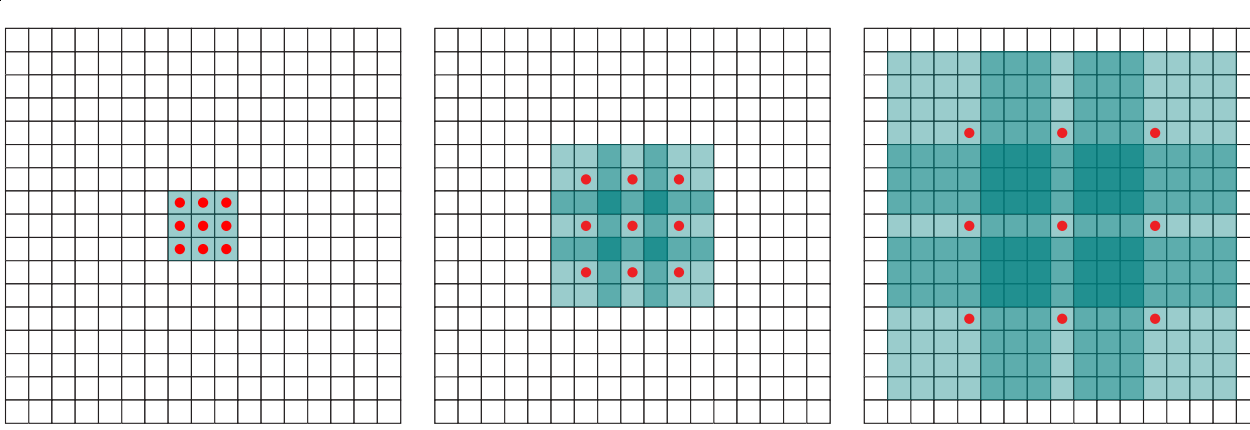
Here we perform convolution with kernel size of 3 (3x3). First image show that all neighbour pixel participate in calculating output. Second image takes every 2nd input (that is, dilate input) and we speak about dilation rate (or factor) of 2. Third image takes every 4th, dilation rate is 4. Regular convolutions take every 1st (all) inputs so dilation rate is 1.
One can think about dilated convolutions as expanding filter weight matrix with zeros interspersing actual weights.

The reason we need such convolutions is receptive field size increase. 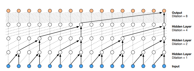 One way to think about stacking dilated convolution layers with exponentially increasing dilation rate is that every subsequent layer doubles (well, almost) receptive field size. That way allows receptive field to grow exponentially rather that linearly.
Consider the very last output (leftmost orange circle) in top layer (one with dilation = 8). It ‘sees’ 8 + 1 outputs (though ignoring 7 of them) so that increases previous layer receptive field size by 8 (not 9 because of kernel width of only 2). Previous layer receptive field size is 8, so it doubled it. Ultimately, it has access to (receptive field size equal to) 16 ground truth samples (blue ones on a pic). Had we hadn’t use dilations we’ll end up with only 5. 8 and 5 are not that big to notice and appreciate the difference but with dilation we get exponential growth rate instead of linear.
This is formula you can use to calculate receptive field size (depends on layers count and stacks count): \(size = stack\_num * (2 ^ {layers\_num + 1})\). Please note, it’s only valid for stride = 1, kernel width = 2.
\(\mu\)-law
Authors use categorical distribution of output amplitudes as was done in PixelCNN. Input data is 16 bit PCM, so output softmax would end up having 65536 categories. In order to decrease computational cost \(\mu\)-law encoding was used (wiki). This transformation takes input in [-1; 1] range and produces output within exactly same range but slightly changes distribution making it more uniform.
First image displays normalized (converted from 16bit integers to floats within [0;1] range) sample value distribution of VCTK p225_001.wav file. Second - same distribution after applying \(\mu\)-law.
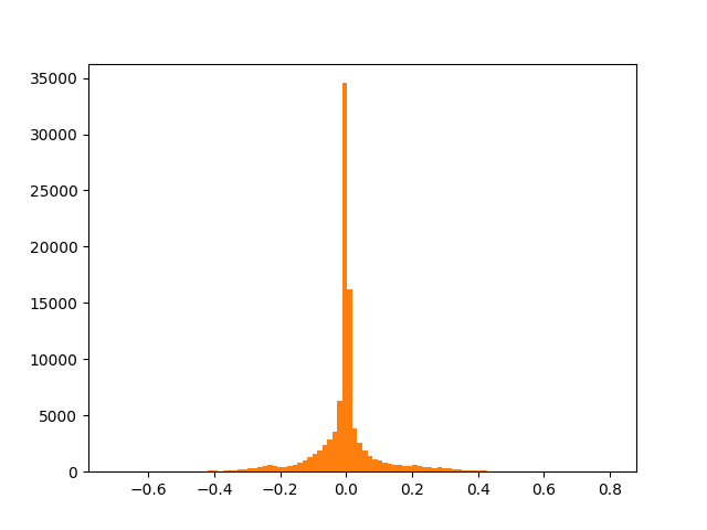
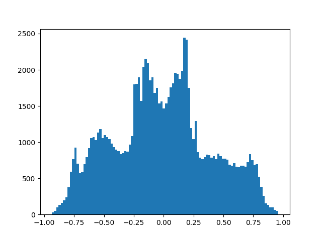
Apparently, \(\mu\)-law encoding places more emphasize on values that are close to zero: it has more granularity for smaller values.
Architecture
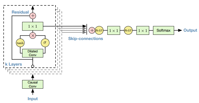
The overall architecture is quite simple (given you have encountered it in PixelCNN):
- First layer mask ‘A’ causal convoluition
- Several stack of layers with dilated convolutions and gated blocks
- Skip connections
- Relu, 1x1 conv, relu, 1x1 conv, softmax
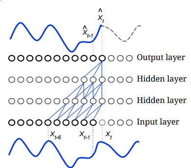
Something I want to emphasize here: Don’t forget about causality in the very first layer! You have to break information flow from sample being predicted and your network. Again, Reed helps here as well (note \(x_t\) and \(\hat{x_t}\) aren’t connected):
Other thing to be ready to is that resildual and skip connections use different 1x1 convolution layers (and weights) after gated block. Skip connections tend to require more channels (filters) rather than residual (i.e. 256 vs 32).

Data preparation
For training you will need some audio data (or any 1D signal, for example stocks or whatever).
The trick to remember is that output signal depends on previous receptive_field_size samples, so while training you should be aware of that. For example, the very first predicted sample would be calculated using zeros as input (because of padding with zeros in all layers). Idea here is to calculate loss only for those samples that are conditioned of already visible signal. Here is visual explaination.

Image abowe shows that only three last outputs (out of 11) have all needed information (1 stack with 3 dilation layers has receptive field size of 8). During loss calculation we ignore all samples that don’t have enough information to calulate meaningful value. For instance, given our sample consists of these 11 inputs, our loss function would be calculated only with regard to L-2, L-1, L outputs.
Data preprocessing step should also incorporate receptive_field_size information as it splits input audio file into chunks and we do want to train with as much information as possible. It’s really easy to see that all we need to do is have an overlap of chunk_length - receptive_field_size for subsequent chunks:

Here, R stands for receptive_field_size, S - data split step size. T is a number of output that will contribute to loss at every sample. Python code snippet should help to grasp that idea:
# our receptive field size
R = 1024
# number of outputs in one sample as well as step
T = 4096
# each sample total length
size = R + T
# step (or stride), equals to T
step = size - R

# our input wav file
audio = np.random.rand(2 ** 20)

while len(audio) > size:
    yield audio[:size]
    audio = audio[step:]
Results
During writing this post I was in the middle of playing and training with a model so my best (I hope so) results await me somewhere in the future.
However, I have some results that I’ve saved during validating model works. Very first result is to try to overfit the model on something very simple. For that purpose I used simple 500Hz tone (sine wave with only one frequency). Laugh not, but even that step required some time for fixing subtle stuff for model, data preprocessing and even training process.
It’s very short (only 4096 samples with 8000 rate, less than half a second), but naive generation implementation took couple of minutes to produce that.
Next result was obtained using VCTK dataset p225 speaker dataset. I trained the model for 24 hours with NVIDIA GTX Titan X, with 4 stacks and 10 layers per stack. Other parameters were default.
Though it doesn’t resemble any human language and talk I really glad it’s not a noise but at least something!
What’s next
Astute reader could note that there is no neither local nor global conditioning. These are nice feature to have but my next milestone is to get model trained on whole dataset and produce even more impressive (for me, of course) results.
SampleRNN authors reconstructed wavenet and report it took them 1 week to train wavenet with 4 stacks and 10 layers on a Blizzard dataset on one NVIDIA Titan X (I don’t know what exact GPU they’ve used). I personally think I won’t surpass their results anyway and will move on to next shiny thing next :)
Also, a very nice paper came from Baidu research group that sounds very promising as it accelerated generation by factor of 400x. Very impressive.
References
Again, helpful and inspiring links (I’m not including original DeepMind paper because it could more helpful and inspiring, instead its intentions are to cipher how while boast about what):
- SampleRNN
- SampleRNN repo
- Deep voice
ibabimplementation, guy from DeepMind